This is “The Observed Significance of a Test”, section 8.3 from the book Beginning Statistics (v. 1.0). For details on it (including licensing), click here.
For more information on the source of this book, or why it is available for free, please see the project's home page. You can browse or download additional books there.


8.3 The Observed Significance of a Test
Learning Objectives
- To learn what the observed significance of a test is.
- To learn how to compute the observed significance of a test.
- To learn how to apply the p-value approach to hypothesis testing.
The Observed Significance
The conceptual basis of our testing procedure is that we reject H0 only if the data that we obtained would constitute a rare event if H0 were actually true. The level of significance specifies what is meant by “rare.” The observed significance of the test is a measure of how rare the value of the test statistic that we have just observed would be if the null hypothesis were true. That is, the observed significance of the test just performed is the probability that, if the test were repeated with a new sample, the result of the new test would be at least as contrary to H0 and in support of Ha as what was observed in the original test.
Definition
The observed significance or p-valueThe probability, if H0 is true, of obtaining a result as contrary to H0 and in favor of Ha as the result observed in the sample data. of a specific test of hypotheses is the probability, on the supposition that H0 is true, of obtaining a result at least as contrary to H0 and in favor of Ha as the result actually observed in the sample data.
Think back to Note 8.27 "Example 4" in Section 8.2 "Large Sample Tests for a Population Mean" concerning the effectiveness of a new pain reliever. This was a left-tailed test in which the value of the test statistic was −1.886. To be as contrary to H0 and in support of Ha as the result actually observed means to obtain a value of the test statistic in the interval Rounding −1.886 to −1.89, we can read directly from Figure 12.2 "Cumulative Normal Probability" that Thus the p-value or observed significance of the test in Note 8.27 "Example 4" is 0.0294 or about 3%. Under repeated sampling from this population, if H0 were true then only about 3% of all samples of size 50 would give a result as contrary to H0 and in favor of Ha as the sample we observed. Note that the probability 0.0294 is the area of the left tail cut off by the test statistic in this left-tailed test.
Analogous reasoning applies to a right-tailed or a two-tailed test, except that in the case of a two-tailed test being as far from 0 as the observed value of the test statistic but on the opposite side of 0 is just as contrary to H0 as being the same distance away and on the same side of 0, hence the corresponding tail area is doubled.
Computational Definition of the Observed Significance of a Test of Hypotheses
The observed significance of a test of hypotheses is the area of the tail of the distribution cut off by the test statistic (times two in the case of a two-tailed test).
Example 6
Compute the observed significance of the test performed in Note 8.28 "Example 5" in Section 8.2 "Large Sample Tests for a Population Mean".
Solution:
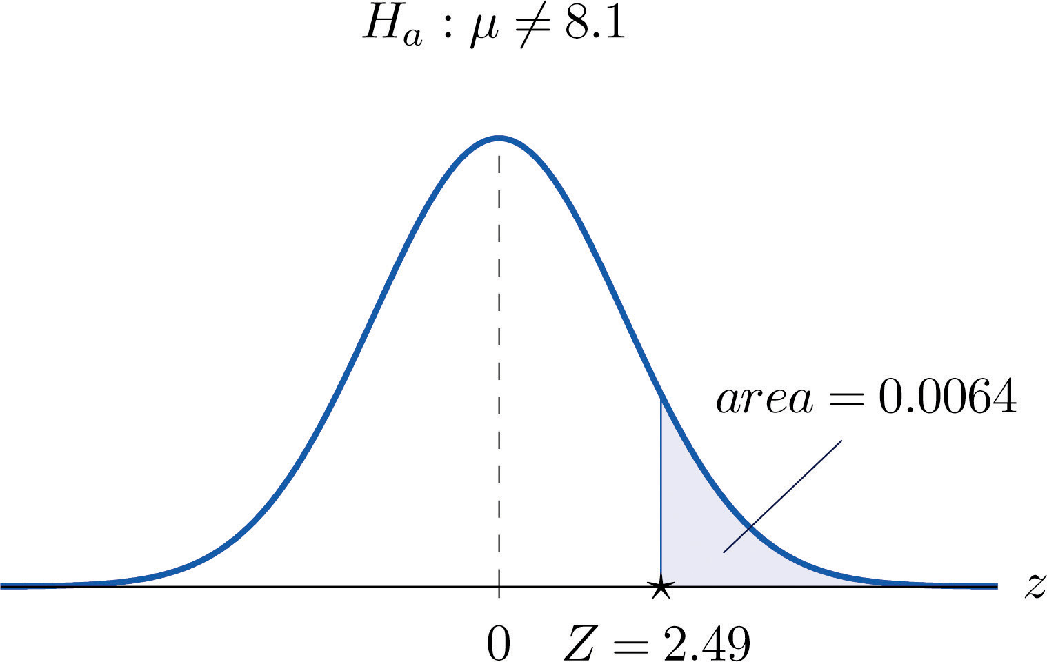
The value of the test statistic was z = 2.490, which by Figure 12.2 "Cumulative Normal Probability" cuts off a tail of area 0.0064, as shown in Figure 8.7 "Area of the Tail for ". Since the test was two-tailed, the observed significance is
Figure 8.7 Area of the Tail for Note 8.34 "Example 6"
The p-value Approach to Hypothesis Testing
In Note 8.27 "Example 4" in Section 8.2 "Large Sample Tests for a Population Mean" the test was performed at the 5% level of significance: the definition of “rare” event was probability or less. We saw above that the observed significance of the test was p = 0.0294 or about 3%. Since (or 3% is less than 5%), the decision turned out to be to reject: what was observed was sufficiently unlikely to qualify as an event so rare as to be regarded as (practically) incompatible with H0.
In Note 8.28 "Example 5" in Section 8.2 "Large Sample Tests for a Population Mean" the test was performed at the 1% level of significance: the definition of “rare” event was probability or less. The observed significance of the test was computed in Note 8.34 "Example 6" as p = 0.0128 or about 1.3%. Since (or 1.3% is greater than 1%), the decision turned out to be not to reject. The event observed was unlikely, but not sufficiently unlikely to lead to rejection of the null hypothesis.
The reasoning just presented is the basis for a slightly different but equivalent formulation of the hypothesis testing process. The first three steps are the same as before, but instead of using to compute critical values and construct a rejection region, one computes the p-value p of the test and compares it to , rejecting H0 if and not rejecting if
Systematic Hypothesis Testing Procedure: p-Value Approach
- Identify the null and alternative hypotheses.
- Identify the relevant test statistic and its distribution.
- Compute from the data the value of the test statistic.
- Compute the p-value of the test.
- Compare the value computed in Step 4 to significance level and make a decision: reject H0 if and do not reject H0 if Formulate the decision in the context of the problem, if applicable.
Example 7
The total score in a professional basketball game is the sum of the scores of the two teams. An expert commentator claims that the average total score for NBA games is 202.5. A fan suspects that this is an overstatement and that the actual average is less than 202.5. He selects a random sample of 85 games and obtains a mean total score of 199.2 with standard deviation 19.63. Determine, at the 5% level of significance, whether there is sufficient evidence in the sample to reject the expert commentator’s claim.
Solution:
-
Step 1. Let μ be the true average total game score of all NBA games. The relevant test is
-
Step 2. The sample is large and the population standard deviation is unknown. Thus the test statistic is
and has the standard normal distribution.
-
Step 3. Inserting the data into the formula for the test statistic gives
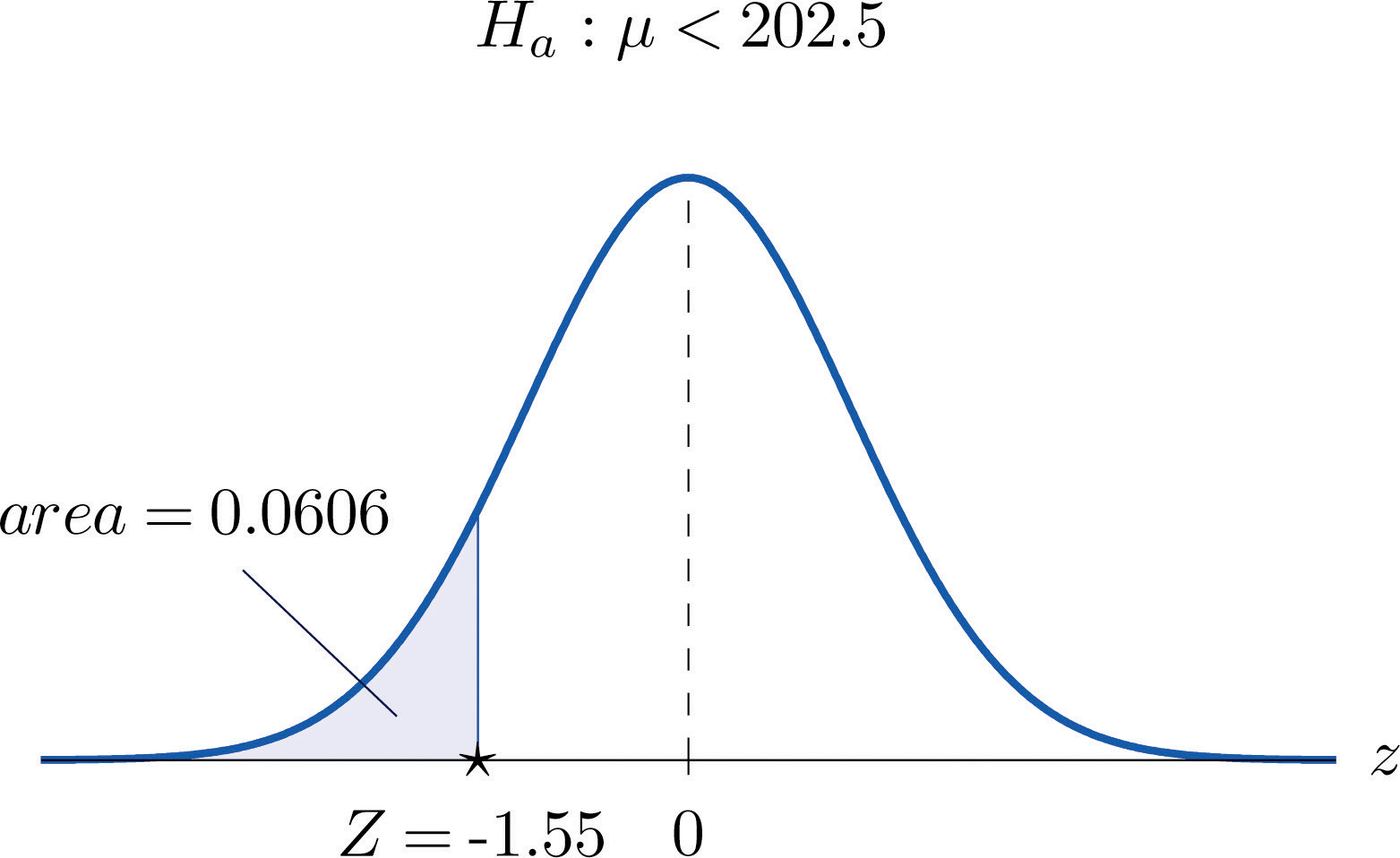
- Step 4. The area of the left tail cut off by is, by Figure 12.2 "Cumulative Normal Probability", 0.0606, as illustrated in Figure 8.8 "Test Statistic for ". Since the test is left-tailed, the p-value is just this number, p = 0.0606.
-
Step 5. Since , the decision is not to reject H0. In the context of the problem our conclusion is:
The data do not provide sufficient evidence, at the 5% level of significance, to conclude that the average total score of NBA games is less than 202.5.
Figure 8.8 Test Statistic for Note 8.36 "Example 7"
Example 8
Mr. Prospero has been teaching Algebra II from a particular textbook at Remote Isle High School for many years. Over the years students in his Algebra II classes have consistently scored an average of 67 on the end of course exam (EOC). This year Mr. Prospero used a new textbook in the hope that the average score on the EOC test would be higher. The average EOC test score of the 64 students who took Algebra II from Mr. Prospero this year had mean 69.4 and sample standard deviation 6.1. Determine whether these data provide sufficient evidence, at the 1% level of significance, to conclude that the average EOC test score is higher with the new textbook.
Solution:
-
Step 1. Let μ be the true average score on the EOC exam of all Mr. Prospero’s students who take the Algebra II course with the new textbook. The natural statement that would be assumed true unless there were strong evidence to the contrary is that the new book is about the same as the old one. The alternative, which it takes evidence to establish, is that the new book is better, which corresponds to a higher value of μ. Thus the relevant test is
-
Step 2. The sample is large and the population standard deviation is unknown. Thus the test statistic is
and has the standard normal distribution.
-
Step 3. Inserting the data into the formula for the test statistic gives
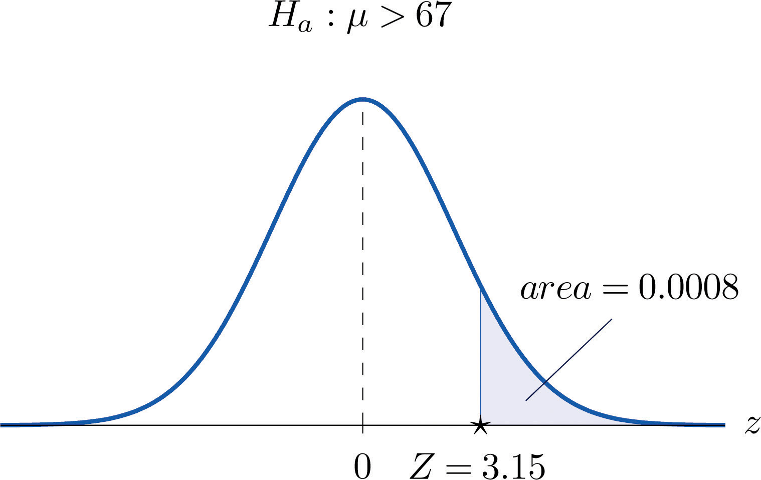
- Step 4. The area of the right tail cut off by z = 3.15 is, by Figure 12.2 "Cumulative Normal Probability", , as shown in Figure 8.9 "Test Statistic for ". Since the test is right-tailed, the p-value is just this number, p = 0.0008.
-
Step 5. Since , the decision is to reject H0. In the context of the problem our conclusion is:
The data provide sufficient evidence, at the 1% level of significance, to conclude that the average EOC exam score of students taking the Algebra II course from Mr. Prospero using the new book is higher than the average score of those taking the course from him but using the old book.
Figure 8.9 Test Statistic for Note 8.37 "Example 8"
Example 9
For the surface water in a particular lake, local environmental scientists would like to maintain an average pH level at 7.4. Water samples are routinely collected to monitor the average pH level. If there is evidence of a shift in pH value, in either direction, then remedial action will be taken. On a particular day 30 water samples are taken and yield average pH reading of 7.7 with sample standard deviation 0.5. Determine, at the 1% level of significance, whether there is sufficient evidence in the sample to indicate that remedial action should be taken.
Solution:
-
Step 1. Let μ be the true average pH level at the time the samples were taken. The relevant test is
-
Step 2. The sample is large and the population standard deviation is unknown. Thus the test statistic is
and has the standard normal distribution.
-
Step 3. Inserting the data into the formula for the test statistic gives
- Step 4. The area of the right tail cut off by z = 3.29 is, by Figure 12.2 "Cumulative Normal Probability", , as illustrated in Figure 8.10 "Test Statistic for ". Since the test is two-tailed, the p-value is the double of this number,
-
Step 5. Since , the decision is to reject H0. In the context of the problem our conclusion is:
The data provide sufficient evidence, at the 1% level of significance, to conclude that the average pH of surface water in the lake is different from 7.4. That is, remedial action is indicated.
Figure 8.10 Test Statistic for Note 8.38 "Example 9"

Key Takeaways
- The observed significance or p-value of a test is a measure of how inconsistent the sample result is with H0 and in favor of Ha.
- The p-value approach to hypothesis testing means that one merely compares the p-value to instead of constructing a rejection region.
- There is a systematic five-step procedure for the p-value approach to hypothesis testing.
Exercises
-
Compute the observed significance of each test.
- Testing vs. , test statistic
- Testing vs. , test statistic
- Testing vs. , test statistic z = 2.54.
-
Compute the observed significance of each test.
- Testing vs. , test statistic z = 2.82.
- Testing vs. , test statistic
- Testing vs. , test statistic z = 1.93.
-
Compute the observed significance of each test. (Some of the information given might not be needed.)
- Testing vs. ; n = 49, , s = 3.14, test statistic z = 3.12.
- Testing vs. ; n = 32, , s = 47.8, test statistic
- Testing vs. ; n = 44, , s = 2.45, test statistic
-
Compute the observed significance of each test. (Some of the information given might not be needed.)
- Testing vs. ; n = 34, , s = 0.87, test statistic
- Testing vs. ; n = 56, , s = 4.82, test statistic z = 2.95.
- Testing vs. ; n = 152, , s = 7.5, test statistic z = 3.29.
-
Make the decision in each test, based on the information provided.
- Testing vs. @ , observed significance p = 0.038.
- Testing vs. @ , observed significance p = 0.038.
-
Make the decision in each test, based on the information provided.
- Testing vs. @ , observed significance p = 0.062.
- Testing vs. @ , observed significance p = 0.062.
Basic
-
A lawyer believes that a certain judge imposes prison sentences for property crimes that are longer than the state average 11.7 months. He randomly selects 36 of the judge’s sentences and obtains mean 13.8 and standard deviation 3.9 months.
- Perform the test at the 1% level of significance using the critical value approach.
- Compute the observed significance of the test.
- Perform the test at the 1% level of significance using the p-value approach. You need not repeat the first three steps, already done in part (a).
-
In a recent year the fuel economy of all passenger vehicles was 19.8 mpg. A trade organization sampled 50 passenger vehicles for fuel economy and obtained a sample mean of 20.1 mpg with standard deviation 2.45 mpg. The sample mean 20.1 exceeds 19.8, but perhaps the increase is only a result of sampling error.
- Perform the relevant test of hypotheses at the 20% level of significance using the critical value approach.
- Compute the observed significance of the test.
- Perform the test at the 20% level of significance using the p-value approach. You need not repeat the first three steps, already done in part (a).
-
The mean score on a 25-point placement exam in mathematics used for the past two years at a large state university is 14.3. The placement coordinator wishes to test whether the mean score on a revised version of the exam differs from 14.3. She gives the revised exam to 30 entering freshmen early in the summer; the mean score is 14.6 with standard deviation 2.4.
- Perform the test at the 10% level of significance using the critical value approach.
- Compute the observed significance of the test.
- Perform the test at the 10% level of significance using the p-value approach. You need not repeat the first three steps, already done in part (a).
-
The mean increase in word family vocabulary among students in a one-year foreign language course is 576 word families. In order to estimate the effect of a new type of class scheduling, an instructor monitors the progress of 60 students; the sample mean increase in word family vocabulary of these students is 542 word families with sample standard deviation 18 word families.
- Test at the 5% level of significance whether the mean increase with the new class scheduling is different from 576 word families, using the critical value approach.
- Compute the observed significance of the test.
- Perform the test at the 5% level of significance using the p-value approach. You need not repeat the first three steps, already done in part (a).
-
The mean yield for hard red winter wheat in a certain state is 44.8 bu/acre. In a pilot program a modified growing scheme was introduced on 35 independent plots. The result was a sample mean yield of 45.4 bu/acre with sample standard deviation 1.6 bu/acre, an apparent increase in yield.
- Test at the 5% level of significance whether the mean yield under the new scheme is greater than 44.8 bu/acre, using the critical value approach.
- Compute the observed significance of the test.
- Perform the test at the 5% level of significance using the p-value approach. You need not repeat the first three steps, already done in part (a).
-
The average amount of time that visitors spent looking at a retail company’s old home page on the world wide web was 23.6 seconds. The company commissions a new home page. On its first day in place the mean time spent at the new page by 7,628 visitors was 23.5 seconds with standard deviation 5.1 seconds.
- Test at the 5% level of significance whether the mean visit time for the new page is less than the former mean of 23.6 seconds, using the critical value approach.
- Compute the observed significance of the test.
- Perform the test at the 5% level of significance using the p-value approach. You need not repeat the first three steps, already done in part (a).
Applications
Answers
-
-
-
-
-
- reject H0
- do not reject H0
-
-
- Z = 3.23, , reject H0
- reject H0
-
-
- Z = 0.68, , do not reject H0
- do not reject H0
-
-
- Z = 2.22, , reject H0
- reject H0
-